Quick Start Guide

This section goes over a quick example of using CryoViT to segment mitochondria in a group of Cryo-ET tomograms using a pre-trained model.

Note

This guide assumes you have already installed CryoViT by following the instructions in Installing CryoViT. If you have not done so, please do that first.

You do not need a working installation of napari to follow this guide, but a GPU is recommended for faster inference.

First, download the example data from here and its contents:

$ tar -xzf example_data.tar.gz

This will extract a directory example_data containing a folder of tomograms data/ and a pre-trained model file pretrained_model.model.

Viewing Tomogram Data

CryoViT supports most common file formats for tomogram data, including .mrc, .tiff, and .hdf formats, expecting the tomogram data to be stored as a 3D array with shape (D, H, W).

You can preview the tomogram data with cryovit.utils.load_data(), which returns the data as a numpy array:

Tip

For .hdf files, which can contain multiple keyed datasets, you can specify which dataset to load by passing in the key argument to cryovit.utils.load_data().

Otherwise, the dataset with the most unique values will be loaded by default, and cryovit.utils.load_data() will return the key found.

>>> from cryovit.utils import load_data
>>> data, key = load_data("example_data/data/HD_iPSC_sample_bin4.hdf")
>>> data
array([[[[0.69411767, 0.5647059 , 0.62352943, ..., 0.49411765,
      0.50980395, 0.47843137],
     [0.5921569 , 0.63529414, 0.6509804 , ..., 0.49803922,
      0.5058824 , 0.50980395],
     [0.6       , 0.6627451 , 0.56078434, ..., 0.5254902 ,
      0.4862745 , 0.5058824 ],
     ...,
     [0.5019608 , 0.5019608 , 0.49019608, ..., 0.50980395,
      0.4745098 , 0.49411765],
     [0.49803922, 0.5058824 , 0.5058824 , ..., 0.49411765,
      0.49411765, 0.52156866],
     [0.49803922, 0.49803922, 0.5019608 , ..., 0.4745098 ,
      0.5411765 , 0.49411765]]]],
  shape=(1, 128, 512, 512), dtype=float32)
>>> key
'data'
>>> print(type(data))
<class 'numpy.ndarray'>
>>> print(data.shape)
(1, 128, 512, 512)  # load_data adds an additional channel dimension
>>> print(data.dtype.name)
float32

Viewing Model Information

CryoViT uses a custom file extension .model to save pre-trained model weights and metadata about the model. You can view the model data with cryovit.utils.load_model(), which returns a tuple containing the model (a pytorch model), and its metadata.

Tip

If you only want to view the metadata without loading the model, you can pass in the argument load_model=False to cryovit.utils.load_model().

>>> from cryovit.utils import load_model
>>> model, model_type, name, label = load_model("example_data/pretrained_mito.model")
>>> print(model)
CryoVIT(
    (metric_fns): ModuleDict(
        ...
    )
    (layers): Sequential(
        ...
    )
    (output_layer): Sequential(
        ...
    )
)
>>> print(model_type)
ModelType.CRYOVIT
>>> print(name)
pretrained_mito
>>> print(label)
mito

We see that the model_type is ModelType.CRYOVIT, indicating that this is a CryoViT segmentation model, and the label is mito, indicating that this model segments mitochondria.

Running Inference Script

The main utilities of CryoViT can be run through command-line scripts. You can see all available scripts by running:

$ cryovit --help
# or
$ cryovit

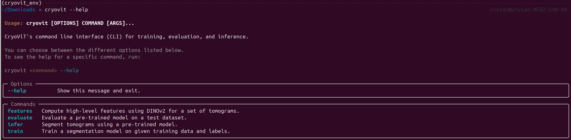
Output of cryovit --help command.

and the arguments for a specific script by running:

$ cryovit <script_name> --help
# or
$ cryovit <script_name>

We see the available scripts are features, train, evaluate, and inference. For this quick start guide, we will be using the inference script to segment the tomograms using the pre-trained model.

Important

Since the model is a CryoViT model, we need to run the features script first to extract the high-level ViT features from the tomograms.

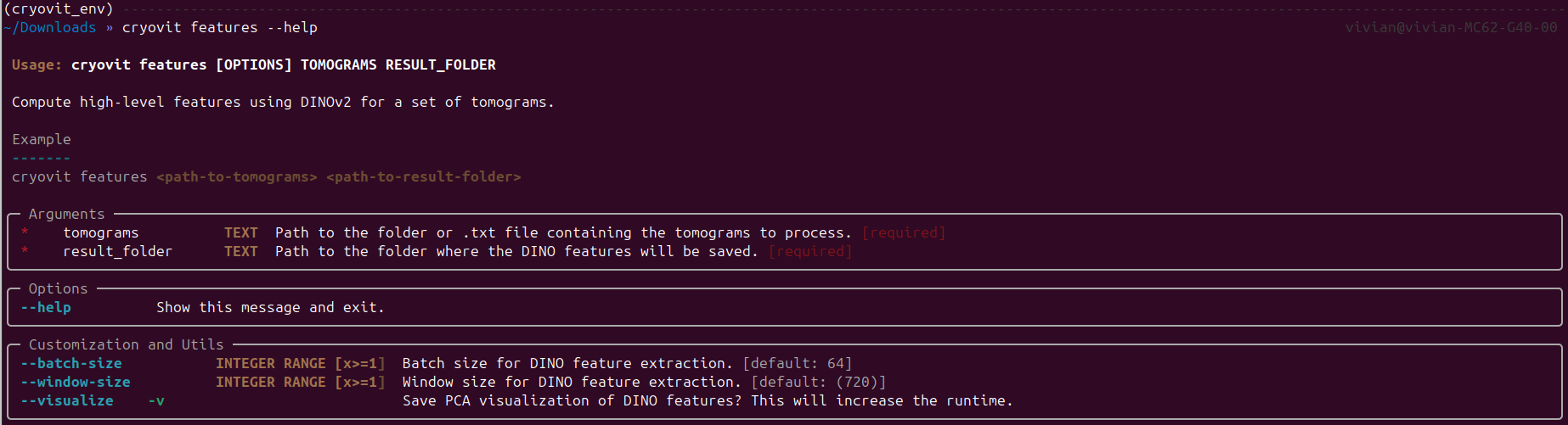
Output of cryovit features --help command.

To run the features script, we need to specify the input tomogram folder and the output directory to save the extracted features:

$ cryovit features example_data/data example_data/features

Note

This step requires a GPU, and is possibly very memory-intensive. If you run into out-of-memory issues, try reducing the --batch-size or --window-size arguments. Reducing the batch size is preferable, as reducing the window size will affect the quality of the extracted features.

Then, we can run the infer script on the extracted features, storing the results in a predictions folder:

$ cryovit infer example_data/features --model example_data/pretrained_model.model --result-folder example_data/predictions

Viewing Segmentation Results

The segmentation results will be saved as .hdf files in the example_data/predictions folder, each containing a data dataset with the original data, and a <label>_preds dataset with the predicted segmentation masks.

While you can still load the predicted segmentations using cryovit.utils.load_data() or cryovit.utils.load_labels(), it is recommended to use a visualization tool like ChimeraX to view the results in 3D, as shown below:

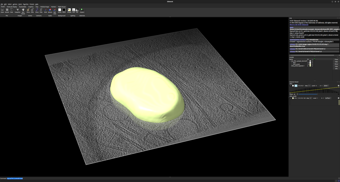
Visualization of tomogram and segmentation results in ChimeraX.